Introduction

The method used for the calculation simplifies the flow as one-dimensional along the mean tank axis and assumes the incompressibility of the fluid [1, 2]. In general a transient flow is considered. The air flow above the fluid is important and is treated as well.

Due to these simplifications, no flow details such as breaking waves or flow separation can be considered. To capture these effects, much more time consuming methods would be needed (approximately more than 1000 times slower). The large amount of computing time makes these methods unattractive for the combination with seakeeping codes. The selected method uses a simple approach and saves computational time. Empirical stationary pressure drop factors describe the viscous effects. The fluid surface is assumed to be nearly perpendicular to the mean tank axis. The conservation equations are applied in integral form resulting in a finite volume method. The tank domain is subdivided with finite control volumes and the complete tank up to its top is modelled. The time is subdivided in time steps.

At both tank tops (tank ends) the pressure is given as boundary condition. This can be e.g. the ambient pressure if free flow through these ends is assumed. It is assumed that valves are fitted to the tank tops, which can be opened and closed by a control mechanism to regulate the air flow. Two types of valve control modes are considered: passive and active control.

The passive valve control mode avoids the sloshing of the fluid against the tank tops. For this purpose, the valve of the non-endangered tank side is closed. The air volume of the most empty tank side then acts as a gas spring and, therefore, the theory of an ideal gas is applied assuming isentropic behaviour. In this case the fluid flow is nearly suppressed. According to the pressure in the ”air buffer”, the pressure boundary condition at this tank end is set. At the endangered tank end, the pressure is set to ambient pressure. Even if the fluid in the tank is idealised as incompressible, the application of the pressure condition in the simulation results in a behaviour in which the air compressibility is taken into account. The valve closes if the fluid level is higher than a certain value below tank top.

The active valve control under certain flow conditions, close the valves, preventing the fluid flow and keeping it on the advantageous side. This can increase the damping at frequencies lower than the resonance frequency, see [1].

Application

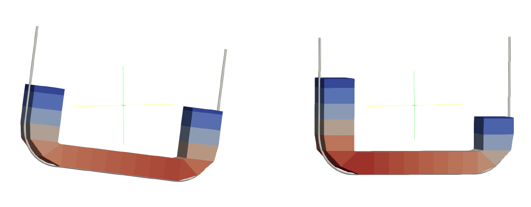
The U-Tank module is used to define the tank geometry and flow parameters. Wizards help to design the tank correctly and adapt the geometry to the ship’s hull. Figure 1 shows an example of the discretised fluid domain.

Results

For Rolf calculations, the tank geometry is automatically integrated and the flow is simulated in the same way as the roll motion. The tank moment m, caused by the moving water mass is determined and added to the roll equation.

For Strip, preliminary calculations are required to integrate the results into the frequency domain. In order incorporate easily the calculated tank moment in the linear strip method the tank moment m′ is defined. In doing so the mass matrix of the ship used in the program does not have to be modified for the tank. The tank moment m′ is the total tank moment m subtracted by the moment produced by the ”frozen” fluid. The frozen fluid with initial position at rest represents the moment in the tank if the fluid does not move relative to the tank. The remaining moment m′ then describes the differences between the total moment due to the movable fluid and the moment due to the frozen fluid taken into account elsewhere.

Many computations with a tank were carried out, covering different roll amplitudes and frequencies. During these simulations the tank oscillates with respect to an assumed roll-axis fixed on the ship. The roll angle φ of the tank is

with angular frequency ω of the roll motion. Every single computation leads to a time history of the roll moment m′ of the tank. This signal is decomposed with a Fourier analysis to

where A₁ is the amplitude of the damping part with a phase shift of 90° relative to the roll angle. Effects of the hydrodynamic mass and the stability loss due to the free surface are summed up in B₁.

In the linear strip program the amplitudes A₁ and B₁ are added to the equation of motion in order to include the tank effect.

As the functions A₁ and B₁ dependent strongly on the roll amplitude due to the non-linear behaviour of the tank effect, the strip method calculations have to be performed for several and suitable roll amplitudes. Figure 2 shows an example of a flow animation.

References

[1] Schumann C., Pereira R.: Non-linear effects of roll damping tanks on ship motions, OMAE2006-92244, pp. 291-300, 25th International Conference on Offshore Mechanics and Arctic Engineering, Hamburg, Germany, 2006.

[2] Schumann C.: Ein Programm zur Berechnung der Strömung in Frahm’schen Schlingerdämpfungstanks; Report No. 627 TU Hamburg-Harburg, Schriftenreihe Schiffbau, February 2004.